Solve the Stokes equation of colliding flow: vector Laplacian version
Synopsis: Compute the solution of the Stokes equation of two-dimensional incompressible viscous flow for a manufactured problem of colliding flow. Hood-Taylor triangular elements are used.
The "manufactured" colliding flow example from Elman et al 2014. The Hood-Taylor formulation with quadratic triangles for the velocity and continuous pressure on linear triangles.
The pressure is shown here with contours, and the velocities visualized with arrows at random points. 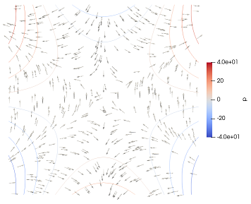
The formulation is the one derived in Donea, Huerta, Introduction to the finite element method, 1993. Page 486 ff, and Elman, et al., Finite elements and fast iterative solvers, p. 132. In brief, it is the vector Laplacian version.
The complete code is in the file tut_stokes_ht_p2_p1_veclap.jl.
The solution will be defined within a module in order to eliminate conflicts with data or functions defined elsewhere.
module tut_stokes_ht_p2_p1_veclapWe'll need some functionality from linear algebra, static arrays, and the mesh libraries. Some plotting will be produced to visualize structure of the stiffness matrix. Finally we will need the Elfel functionality.
using LinearAlgebra
using StaticArrays
using MeshCore.Exports
using MeshSteward.Exports
using Elfel.Exports
using UnicodePlots
The boundary value problem is expressed in this weak form
\[ \int_{V}\mu {\underline{\nabla}}\;\underline{\delta v}\; :\; {\underline{\nabla}}\;\underline{u}\; \mathrm{d} V - \int_{V} \mathrm{div}(\underline{\delta v})\; p\; \mathrm{d} V = 0,\quad \forall \underline{\delta v}\]
\[ - \int_{V} \delta q\; \mathrm{div}(\underline{u}) \; \mathrm{d} V = 0,\quad \forall \delta q\]
Here $\underline{\delta v}$ are the test functions in the velocity space, and $\delta q$ are the pressure test functions. Further $\underline {u}$ is the trial velocity, and $p$ is the trial pressure. The operator $:$ produces the componentwise scalar product of the gradients,
\[A\; :\;B = A_{ij}B_{ij}``.\]
Then the first term may be rewritten as
\[{\underline{\nabla}}\;\underline{\delta v}\; :\; {\underline{\nabla}}\;\underline{u} = (\underline{\nabla}\delta v_x)^T \underline{\nabla}u_x + (\underline{\nabla}\delta v_y)^T \underline{\nabla}u_y\]
function run()
    mu = 1.0 # dynamic viscosity
    A = 1.0 # half of the length of the side of the square
    N = 100 # number of element edges per side of the square
These three functions define the true velocity components and the true pressure.
    trueux = (x, y) -> 20 * x * y ^ 3
    trueuy = (x, y) -> 5 * x ^ 4 - 5 * y ^ 4
    truep = (x, y) -> 60 * x ^ 2 * y - 20 * y ^ 3
Construct the two meshes for the mixed method. They need to support the velocity and pressure spaces.
vmesh, pmesh = genmesh(A, N)Construct the velocity space: it is a vector space with two components. The degrees of freedom are real numbers (Float64). The velocity mesh carries the finite elements of the continuity $H ^1$, i. e. both the function values and the derivatives are square integrable. Each node carries 2 degrees of freedom, hence there are two velocity components per node.
Uh = FESpace(Float64, vmesh, FEH1_T6(), 2)Now we apply the boundary conditions at the nodes around the circumference.
locs = geometry(vmesh)We use searching based on the presence of the node within a box. The entire boundary will be captured within these four boxes, provided we inflate those boxes with a little tolerance (we can't rely on those nodes to be precisely at the coordinates given, we need to introduce some tolerance).
    boxes = [[-A A -A -A], [-A -A -A A], [A A -A A], [-A A A A]]
    inflate = A / N / 100
    for box in boxes
        vl = vselect(locs; box = box, inflate = inflate)
        for i in vl
Remember that all components of the velocity are known at the boundary.
            setebc!(Uh, 0, i, 1, trueux(locs[i]...))
            setebc!(Uh, 0, i, 2, trueuy(locs[i]...))
        end
    end
No we construct the pressure space. It is a continuous, piecewise linear space supported on a mesh of three-node triangles.
Ph = FESpace(Float64, pmesh, FEH1_T3(), 1)The pressure in this "enclosed" flow example is only known up to a constant. By setting pressure degree of freedom at one node will make the solution unique.
    atcenter = vselect(geometry(pmesh); nearestto = [0.0, 0.0])
    setebc!(Ph, 0, atcenter[1], 1, 0.0)
Number the degrees of freedom. First all the free degrees of freedom are numbered, both velocities and pressures. Next all the data degrees of freedom are numbered, again both for the velocities and for the pressures.
numberdofs!([Uh, Ph])The total number of degrees of freedom is now calculated.
tndof = ndofs(Uh) + ndofs(Ph)As is the total number of unknowns.
tnunk = nunknowns(Uh) + nunknowns(Ph)Assemble the coefficient matrix.
K = assembleK(Uh, Ph, tndof, mu)Display the structure of the indefinite stiffness matrix. Note that this is the complete matrix, including rows and columns for all the degrees of freedom, unknown and known.
    p = spy(K, canvas = DotCanvas)
    display(p)
Solve the linear algebraic system. First construct system vector of all the degrees of freedom, in the first tnunk rows that corresponds to the unknowns, and the subsequent rows are for the data degrees of freedom.
    U = fill(0.0, tndof)
    gathersysvec!(U, [Uh, Ph])
Note that the vector U consists of nonzero numbers in rows are for the data degrees of freedom. Multiplying the stiffness matrix with this vector will generate a load vector on the right-hand side. Otherwise there is no loading, hence the vector F consists of all zeros.
    F = fill(0.0, tndof)
    solve!(U, K, F, tnunk)
Once we have solved the system of linear equations, we can distribute the solution from the vector U into the finite element spaces.
scattersysvec!([Uh, Ph], U)Given that the solution is manufactured, i. e. exactly known, we can calculate the true errors.
    @show ep = evaluate_pressure_error(Ph, truep)
    @show ev = evaluate_velocity_error(Uh, trueux, trueuy)
Postprocessing. First we make attributes, scalar nodal attributes, associated with the meshes for the pressures and the velocity.
    makeattribute(Ph, "p", 1)
    makeattribute(Uh, "ux", 1)
    makeattribute(Uh, "uy", 2)
The pressure and the velocity components are then written out into two VTK files.
    vtkwrite("tut_stokes_ht_p2_p1_veclap-p", baseincrel(pmesh), [(name = "p",), ])
    vtkwrite("tut_stokes_ht_p2_p1_veclap-v", baseincrel(vmesh), [(name = "ux",), (name = "uy",)])
The method converges very well, but, why not, here is the true pressure written out into a VTK file as well. We create a synthetic attribute by evaluating the true pressure at the locations of the nodes of the pressure mesh.
    geom = geometry(Ph.mesh)
    ir = baseincrel(Ph.mesh)
    ir.right.attributes["pt"] = VecAttrib([truep(geom[i]...) for i in 1:length(geom)])
    vtkwrite("tut_stokes_ht_p2_p1_veclap-pt", baseincrel(pmesh), [(name = "pt",), ])

    return true
end

function genmesh(A, N)
Hood-Taylor pair of meshes is needed. The first mesh is for the velocities, composed of six-node triangles.
vmesh = attach!(Mesh(), T6block(2 * A, 2 * A, N, N), "velocity")Now translate so that the center of the square is at the origin of the coordinates.
    ir = baseincrel(vmesh)
    transform(ir, x -> x .- A)
The second mesh is used for the pressures, and it is composed of three-node triangles such that the corner nodes are shared between the first and the second mesh.
pmesh = attach!(Mesh(), T6toT3(baseincrel(vmesh, "velocity")), "pressure")Return the pair of meshes
    return vmesh, pmesh
end

function assembleK(Uh, Ph, tndof, mu)
    function integrate!(ass, elits, qpits, mu)
This array defines the components for the element degrees of freedom: $c(i)$ is 1 or 2.
c = edofcompnt(Uh)These are the totals of the velocity and pressure degrees of freedom per element.
n_du, n_dp = ndofsperel.((Uh, Ph))The local matrix assemblers are used as if they were ordinary elementwise dense matrices. Here they are defined.
        kuu = LocalMatrixAssembler(n_du, n_du, 0.0)
        kup = LocalMatrixAssembler(n_du, n_dp, 0.0)
        for el in zip(elits...)
            uel, pel = el
The local matrix assemblers are initialized with zeros for the values, and with the element degree of freedom vectors to be used in the assembly. The assembler kuu is used for the velocity degrees of freedom, and the assembler kup collect the coupling coefficients between the velocity and the pressure. The function eldofs collects the global numbers of the degrees of freedom either for the velocity space, or for the pressure space (eldofs(pel)).
            init!(kuu, eldofs(uel), eldofs(uel))
            init!(kup, eldofs(uel), eldofs(pel))
            for qp in zip(qpits...)
                uqp, pqp = qp
The integration is performed using the velocity quadrature points.
                Jac, J = jacjac(uel, uqp)
                JxW = J * weight(uqp)
                gradNu = bfungrad(uqp, Jac) # gradients of the velocity basis functions
                Np = bfun(pqp) # pressure basis functions
This double loop corresponds precisely to the integrals of the weak form: dot product of the gradients of the basis functions. This is the matrix in the upper left corner.
                for i in 1:n_du, j in 1:n_du
                    if c[i] == c[j]
                        kuu[j, i] += (mu * JxW) * (dot(gradNu[j], gradNu[i]))
                    end
                end
And this is the coupling matrix in the top right corner.
                for i in 1:n_dp, j in 1:n_du
                    kup[j, i] += gradNu[j][c[j]] * (-JxW * Np[i])
                end
            end
Assemble the matrices. The submatrix off the diagonal is assembled twice, once as itself, and once as its transpose.
            assemble!(ass, kuu)
            assemble!(ass, kup) # top right corner
            assemble!(ass, transpose(kup)) # bottom left corner
        end
        return ass # return the updated assembler of the global matrix
    end
In the assembleK function we first we create the element iterators. We can go through all the elements, both in the velocity finite element space and in the pressure finite element space, that define the domain of integration using this iterator. Each time a new element is accessed, some data are precomputed such as the element degrees of freedom, components of the degree of freedom, etc. Note that we need to iterate two finite element spaces, hence we create a tuple of iterators.
elits = (FEIterator(Uh), FEIterator(Ph))These are the quadrature point iterators. We know that the elements are triangular. We choose the three-point rule, to capture the quadratic component in the velocity space. Quadrature-point iterators provide access to basis function values and gradients, the Jacobian matrix and the Jacobian determinant, the location of the quadrature point and so on. Note that we need to iterate the quadrature rules of two finite element spaces, hence we create a tuple of iterators.
    qargs = (kind = :default, npts = 3,)
    qpits = (QPIterator(Uh, qargs), QPIterator(Ph, qargs))
The matrix will be assembled into this assembler. Which is initialized with the total number of degrees of freedom (dimension of the coefficient matrix before partitioning into unknowns and data degrees of freedom).
    ass = SysmatAssemblerSparse(0.0)
    start!(ass, tndof, tndof)
The integration is carried out, and then...
integrate!(ass, elits, qpits, mu)...we materialize the sparse stiffness matrix and return it.
    return finish!(ass)
end
The linear algebraic system is solved by partitioning. The vector U is initially all zero, except in the degrees of freedom which are prescribed as nonzero. Therefore the product of the stiffness matrix and the vector U are the loads due to nonzero essential boundary conditions. The submatrix of the stiffness conduction matrix corresponding to the free degrees of freedom (unknowns), K[1:nu, 1:nu] is then used to solve for the unknowns U [1:nu].
function solve!(U, K, F, nu)
    KT = K * U
    U[1:nu] = K[1:nu, 1:nu] \ (F[1:nu] - KT[1:nu])
end
The function evaluate_pressure_error evaluates the true $L^2$ error of the pressure. It does that by integrating the square of the difference between the approximate pressure and the true pressure, the true pressure being provided by the truep function.
function evaluate_pressure_error(Ph, truep)
    function integrate!(elit, qpit, truep)
        n_dp = ndofsperel(elit)
        E = 0.0
        for el in elit
            dofvals = eldofvals(el)
            for qp in qpit
                Jac, J = jacjac(el, qp)
                JxW = J * weight(qp)
                Np = bfun(qp)
                pt = truep(location(el, qp)...)
                pa = 0.0
                for j in 1:n_dp
                    pa += (dofvals[j] * Np[j])
                end
                E += (JxW) * (pa - pt)^2
            end
        end
        return sqrt(E)
    end

    elit = FEIterator(Ph)
    qargs = (kind = :default, npts = 3,)
    qpit = QPIterator(Ph, qargs)
    return integrate!(elit, qpit, truep)
end
The function evaluate_velocity_error evaluates the true $L^2$ error of the velocity. It does that by integrating the square of the difference between the approximate pressure and the true velocity, the true velocity being provided by the trueux, trueuy functions.
function evaluate_velocity_error(Uh, trueux, trueuy)
    function integrate!(elit, qpit, trueux, trueuy)
        n_du = ndofsperel(elit)
        uedofcomp = edofcompnt(Uh)
        E = 0.0
        for el in elit
            udofvals = eldofvals(el)
            for qp in qpit
                Jac, J = jacjac(el, qp)
                JxW = J * weight(qp)
                Nu = bfun(qp)
                uxt = trueux(location(el, qp)...)
                uyt = trueuy(location(el, qp)...)
                uxa = 0.0
                uya = 0.0
                for j in 1:n_du
                    (uedofcomp[j] == 1) && (uxa += (udofvals[j] * Nu[j]))
                    (uedofcomp[j] == 2) && (uya += (udofvals[j] * Nu[j]))
                end
                E += (JxW) * ((uxa - uxt)^2 + (uya - uyt)^2)
            end
        end
        return sqrt(E)
    end

    elit = FEIterator(Uh)
    qargs = (kind = :default, npts = 3,)
    qpit = QPIterator(Uh, qargs)
    return integrate!(elit, qpit, trueux, trueuy)
end

end
To run the example, evaluate this file which will compile the module .tut_stokes_ht_p2_p1_veclap.
using .tut_stokes_ht_p2_p1_veclap
tut_stokes_ht_p2_p1_veclap.run()
This page was generated using Literate.jl.